Stabilizing the Renewable Grid
The Off-Peak Energy Market

New wind farms are signing PPAs for energy at $50/MWh, where will you get energy for $15/MWh?
There are numerous points throughout the discussion of WindFuels where we note an expected price for off-peak carbon neutral energy. In the economics discussion, the worst-case energy prices that we project in the near term are $25/MWh, and the average case is $15/MWh. This price expectation is our most often misunderstood claim – and therefore the claim that is most often challenged.

Understanding the effect that deep wind power penetration has on the electricity market is crucial to understanding one of the most exciting advantages of the WindFuels system – its ability to use intermittent renewable energy whenever it is available at a low price.

The ISO/RTO markets.
Most states within the U.S. have their electrical energy traded through virtual markets within an Independent System Operator (ISO) or Regional Transmission Operator (RTO). The energy is openly bought and sold within these virtual markets in short blocks, and the pricing is recorded as Local Marginal Price (LMP) - the amount a buyer would be willing to pay for one additional MWh of energy traded within that time frame.

ISO/RTO systems are more favorable than other structures to wind projects at large, as the larger region of established trade allows for more transmission of energy, “smoothing” local variability. The limit to the expansion of wind is based on its profitability, so wind power typically continues to penetrate until something limits its continued development. In ISO/RTO markets, the limiter is often the final price of energy – which causes power companies to hesitate to sign more Purchase Power Agreements (PPA’s) for delivered energy.

When we first began investigating the economics of the WindFuels system, we focused on the Minnesota hub in MISO (an RTO that includes much of the industrial Northern Midwest). At the time, Minnesota was the state that had the greatest penetration of wind, followed by Iowa and North Dakota. The Minnesota hub sees trades that cover all of MN, ND, and Northern IA. This then was considered an ideal predictor of what an electric market with reasonably high penetration of wind might look like if grid transmission was adequate. We’ve continued tracking this hub. For the rest of this discussion, we will be including data from MISO’s RT trades (wind is typically traded in the real time or RT market) over the Minnesota hub. More dramatic information could be shown from ERCOT data, but in ERCOT transmission issues dominate difficulties with wind power penetration. There are no transmission problems for the Minnesota hub.

End-use consumers see little price difference between peak and off-peak energy, or hour-by hour. End-use customers contract for a given rate, and they use energy as dictated by need. A WindFuels system would differ because it would be available to take its contracted energy needs at times that are solely within the discretion of the energy provider – who is trading over MISO. So most of the Windfuels plant’s energy needs could be satisfied during the cheapest hours of energy on any given day, and the energy provider could benefit from having an easy-to-shed energy load to help deal with sudden price spikes.

This would be a huge benefit for the power company, as it would help draw some of the excess energy off of the grid, forcing the prices higher for the rest of the trades. If the presence of an extra few percent energy beyond demand is forcing RT energy trades to be negatively priced for 7-40 hours/week, then a power company could simply contract with a WindFuels plant for the excess RT energy at a very low price. On some days they'd lose money on that contract, but more often they'd get far more for that energy sold to Windfuels then they would have gotten had they traded it over the ISO (note the “cheapest 6 hours/day” trace in the above graph – its average recent price is about $8/MWh). However, there would now be a market every day with a little less energy traded RT, which would likely lead to much stronger RT prices. Thus they would generate more revenue on the improved pricing for the rest of the RT sales than they could ever lose for the Windfuels contract.

There is no better way in an ISO for a power provider to manipulate supply at that level without substantial losses – in true real time. It’s a question of game theory. If a single power provider tried to manipulate the energy levels through curtailing much more of their wind electricity, that provider would lose 100% of the revenue of their curtailed wind, and the curtailment of other wind farms would quickly be reduced until the RT price was back down to about the same level that it had been (price is causing these providers to determine when they curtail their wind). So any provider trying to be more aggressive about wind curtailment loses more money and advantages their competitors without getting anything back in return. If instead the excess were simply drawn off the grid by a controlled variable load, the wind turbines would see less curtailment and the net prices for the rest of the energy traded would either be the same or higher. The power provider could then gain both in decreased curtailment and in increased nighttime prices.

Negative priced energy?
You may (or may not) have heard of the concept of negative priced energy. But there are times when power companies must literally pay others to take their energy to avoid damage to their assets and those of their customers on the grid.
Negative pricing occurs whenever electricity providers must reduce the net energy on the grid but do not expect to require the energy levels to be reduced for long. Baseload power is slow to ramp up and down, and sees a highly reduced efficiency if it is quickly cycled.

Power companies are continually making decisions on the extent to which their fossil power generation is tamped down versus selling excess energy to their neighbors at prices that may not be profitable. As more and more wind energy is brought online in any region, preferential treatment of local wind power will ensure that local markets would use some of their locally produced wind energy rather than curtailing it, which means that more energy is now supplied in a market that hasn’t seen any change in demand. Most grids have less than 10 minutes worth of battery storage capacity, so supply and demand fundamentals don’t stop affecting prices at production costs, nor do they stop influencing prices at $0/MWh.

While negative pricing is not new, intermittent wind energy has caused the instance of negative energy to increase over the past 4 years. Figure 2 shows the price of energy at every hour during the month of December 2011. While the resolution is limited, different colors were used for days of the week, and different shapes were used for different weeks of the month. The average hourly price for the month is traced. (Note these are hourly averages, actual prices within any given hour can swing wildly from one 5-minute trading block to the next during a period where wind speed is inconstant).

Figure 2 shows a scatter plot of the trade LMP (local marginal price) over the Minnesota hub in the real time market of December 2011. While the average price of energy traded was $23.20/MWh, it is clear from the trace that the average price for any individual hour had a large range, and that many hours were negatively priced.

Negative pricing occurs even in regions that are seeing large curtailment rates. In fact, throughout ERCOT, it is virtually impossible to see a day go by without several hours of negative pricing, even though ERCOT mandates curtailing and the ISO oversees more wind curtailment than any other region in America.

As expected, most of the periods of lowest-priced energy fall within periods of higher wind power generation. As will be explained more fully in the section “Wind Curtailment” below, the instance of negative pricing is quite sensitive to the price of natural gas – with periods of higher cost natural gas resulting in more negative pricing and curtailment, and periods of lower cost natural gas resulting in fewer cases of both of the above.

Figure 3 illustrates the number of hours per quarter that energy has been traded at very low prices (<$10/MWh) and the number of hours per quarter that energy has been traded at negative pricing. The reduction in low and negatively priced energy seen between 2009 and 2010 was a direct result of the fact that the amount of energy curtailed in this region nearly tripled in that time frame. The modest stability that occurred throughout 2011 reflected a balance between dropping natural gas prices and increasing wind power penetration.

Figure 3: The red columns show the number of hours energy prices averaged below $0/MWh throughout the Minnesota hub, the blue columns show the number of hours energy traded below $10/MWh.

As more wind power is installed, more locales will have excess energy more often that they have to sell, increasing the supply in the open market. This serves to increase both the instance of negative energy prices and the amount of wind curtailment.

Wind Curtailment.
An oft-heard criticism of wind farms is that people “drive by them every day while the wind is blowing and the turbines aren’t spinning”. This is true, and it’s often deliberate. The turbine blades are often pitched so that they recover less energy or no energy from the wind, a process commonly referred to as “wind curtailment”. The reason is obvious: if overproduction of wind power results in negative or ultra-low priced energy, one way to avoid paying to get rid of excess energy is shutting down the energy production. So curtailment happens either to prevent or eliminate negative pricing.

When the amount of energy coming online is greater than the energy demand, the power provider must determine whether to reduce wind-energy generation, or ramp down fossil power (it takes 5-10 minutes to tamp down an NG peaker, 15-20 minutes to tamp down a combined cycle gas turbine (CCGT), and hours to tamp down a coal plant). If fossil power is chosen to be tamped back, the price of energy will likely stay negative as long as that process takes.

If the power company backs off too far on a coal plant in the evening, and then the wind suddenly drops, the power company will lose money buying emergency excess power from neighboring markets and pushing their natural gas peaking plants to max, all while inefficiently re-firing their coal plants. The money lost due to such a miscalculation could easily exceed what it would cost the power company to just keep the baseload plants burning and curtail some of the wind when the wind blows strongly. So the power companies use the best weather predictions available (which are very accurate for a time horizon of a few hours,) and make the best choices they can for maximizing profit.

The more wind power penetrates within a given regional grid, the greater this problem becomes, and the greater the instance of curtailment. Clearly, if natural gas is used as the “balance power”, one of the key economic factors becomes the price of natural gas itself. When natural gas prices are low, then the economic penalty of shifting more power from baseload to natural gas is reduced. Baseload is reduced to a greater extent when higher winds are forecast – leading to less curtailment. When NG prices are high, then there is a greater economic penalty for using the balance power, and there would be more instances where the power company will curtail the wind power instead of reducing baseload power.

This is very complex, but in order to offer a visual illustration of these impacts we’ll look specifically at Iowa – a plains state with no hydropower capacity that sits at the convergence of the three largest RTO’s in the U.S.: MISO, PJM, and SPP; so there’s no question of transmission capacity here.

The following graph shows the total amount of wind energy curtailed in Iowa in GWh (red columns), the percentage of Iowa’s generation that was derived from wind (green area), and the price of natural gas in $/MMBTU (black line).

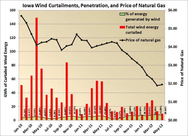
Note that even at NG prices of below $2.00/MMBTU Iowa is still curtailing more than 10 GWh/month. When gas prices were $4/MMBTU, there was 169 GWh of curtailed wind energy because the wind power penetration increased from 14.4% to 17.4%. Currently ~25% of the state’s energy is derived from wind. An increase in natural gas prices should result in far higher curtailment then was seen previously at $4.00/MMBTU, as the wind power percentage of total generation has increased dramatically.

WindFuels would end curtailments.
We expect that a major power provider would have a strong incentive to contract with a WindFuels plant. In cases where excess wind production begins to threaten grid stability, rather than curtailing the wind they could merely direct excess energy to the electrolyzers at a nearby WindFuels facility. This energy would be contracted for a very low price, as the alternative would be curtailment – which has zero value – or actually see the market price go negative. In return, the power company could get SOME return on those hours of wind power rather than none or negative, and they would also be eligible to receive credit for renewable energy generation being delivered to the grid – whether that would serve to satisfy mandates or offer subsidies or tax credits.

There is a beautiful synergy here. If natural gas is cheap, a CARMA plant would derive most of its feedstock from natural gas, while purchasing some grid energy when the power company would otherwise curtail their winds. If natural gas starts increasing in price, the amount of extremely low cost grid energy will increase non-linearly and the CARMA plant can use more cheap grid energy and less NG.

The other advantage for the power company is that there is now the potential for a more stable grid at large, with the power company having the ability to adjust the demand from electrolyzers from 2% to 100% or anywhere in between with <100 millisecond (ms) warning. This would enable them to efficiently plan for operations and run all of their baseload thermal systems at maximum efficiency and effectiveness, while smoothing the way for much greater wind penetration at maintained stability.

There is clearly a strong incentive for power providers to offer very low energy pricing for WindFuels whenever RT prices are very low, and there is enough curtailed wind energy NOW (even with very low-priced natural gas) to provide for the needs of scores of WindFuels plants throughout the Midwest.

Climate Benefit Note: if a new WindFuels plant is brought online within a region and consumes 100 GWh from the grid with specific timing so that there is 100 GWh less wind curtailment, then no additional fossil energy would be used to provide that portion of energy consumed by the WindFuels plant. The actual impact will be greater than this, as a more stable grid requiring less curtailment would encourage more development of wind within a grid – allowing more fossil energy to be abated than could ever have occurred without WindFuels plants being present.

Wasted Electrical Energy.
Keep in mind that during these times of high winds and excess power, power companies are losing money hand over fist. Baseload power costs money, and power companies have to pay the ISOs in order to trade energy, which they are often trading at negative value.

When energy is traded over the ISOs at such times, it is often “purchased” by neighboring municipalities, who now have excess power that they must “sell” at a slightly higher price to their neighbors… in effect a series of fees paid to the ISO to “push” the energy to outlying regions that are not suffering from an energy glut. The transmission may be through lines and transformers that are near capacity, thereby imposing additional costs on the trading.

But other means of dealing with excess energy abound. It’s fairly easy to imagine that every light in every facility owned by a power company will be shining brightly before excess power gets “sold” for a negative price. The same is undoubtedly true with excess AC/climate control, water heating, and whatever else can be done with the energy, including simply running large amounts of energy through resistor banks and heating the parking lots.

If the energy is being “sold” at negative pricing, it’s equally easy to imagine the co-ops who “purchase” this energy would also be motivated to use this energy even if they don’t have sufficient demand within their customer base, and they too would use lighting, heating, air conditioning, and any other power draw they could find to utilize or waste this electricity in the middle of the night.

This is why it is not uncommon to see areas that boast of “green” initiatives end up having tremendous amounts of lights burning in every city building through the night, or large outdoor heating vents operating at odd times throughout the night.
There is no way to determine exactly how much electricity is wasted, but there is a certain financial motivation, and compelling anecdotal evidence throughout the wind corridor.

As wind power continues to build out and develop a deeper penetration into regional grid portfolios, all three of these issues that are currently costing power companies – curtailment, negative energy pricing, and electricity wasting – will continue to increase. A low-cost contract for variable power demand during excess generation periods would be far more profitable for the power companies in all cases. We expect there will be no difficulty getting favorable contracts for at least the next several decades.

Won’t they simply stop building wind farms? The immediate reaction from most investors after they learn about some of the difficulties facing high wind penetration into the grid is: clearly this cannot last! They’ll stop building wind power until some “fix” is found. The DOE apparently agrees with this assessment. However, the DOE’s record of projecting renewable energy installations may be even worse than their record on projecting oil prices, and they have had a history of being irrationally bearish on wind in particular, as we’ll show... Even as recently as early 2008, the DOE’s “high economic growth case” in their Annual Energy Outlook (AEO) 2008 was projecting a total wind capacity of 27.3 GW by 2010 and 34.6 GW by 2020. According to AEO 2008 we would see 94 TWh generated in 2019. The projections for wind energy generation according to the AEO 2011 are shown in Table 1. The boldfaced years represent actual data, the remaining are projections calculated from the 4th quarter of 2010. The actual data from 2010 shows that the year ended with wind generation totaling 94.6 TWh. At the end of the second quarter of 2012, the total installed capacity across America was 50 GW, a milestone that the DOE stated just 16 months earlier would not be reached for another 11 years. While the prediction of a complete cessation of any new installations in wind power may seem shocking, the DOE has been predicting just such an event for years. Each year with the new release of the AEO, they merely advance the year in which all wind growth stops. The DOE’s 2012 AEO has remained true to form, projecting 53 GW of installed wind power by the end of 2012, and 54 GW of installed wind power by the end of 2020. There’s currently another 10 GW of wind power under construction in the U.S., which will certainly be completed within the next 16 months. It seems obvious that this kind of projection is more a reflection of bias at the DOE rather than a serious attempt to project the growth of wind. This may seem to be picking on the DOE excessively, but it is important to realize that they have historically been further afield in their projections for renewable energy than any other analysts, including coal and natural gas lobbies.

Year Average Installed Capacity Total Generation 2008 24.89 55.42 2009 31.45 70.82 2010 37.49 91.25 2011 41.62 109.31 2012 48.9 141.78 2013 48.9 141.77 2014 48.9 141.77 2015 48.9 141.77 2016 48.9 141.77 2017 48.9 141.78 2018 48.9 141.78 2019 48.9 141.78 2020 49.01 142.16 2021 49.01 142.16 2022 49.64 144.32 2023 50.3 146.6 2024 50.78 148.46 2025 51.56 150.73                           Table 1: Unreasonably pessimistic projections from the DOE AEO 2011 for wind development in the U.S.

You still haven’t explained why they won’t just stop building wind farms.
It boils down to government intervention. Thirty-eight states have renewable portfolio standards (RPSs, sometimes called RESs, renewable electricity standards). For these states, the power companies are mandated to utilize more renewable energy, whether there is a cost justification in doing so or not. This has been the dominant driving force behind both the wind and solar industries for the past decade, and more states are either adopting or expanding RPSs every year. After the record-shattering heat wave/drought of 2012, it’s likely that resistance to measures reducing carbon emissions should decrease throughout the wind belt, and even more aggressive RPS legislation may come into play.

Table 2 was compiled (mid-2012) to help give a better appreciation for how much renewable energy must be brought online in the coming years – in order to comply with government mandates. Some RPSs specify installed capacity rather than percentage of energy produced. Many specify minimum portions for certain industries, and in some cases a date is specified so that only newer installations can count towards this mandate.

State	2011 Energy Demand	State RPS Mandate/ Goal	Specified non-wind	Unspecified renewable energy needed to fulfill RPS assuming 0.8% annual growth	Mandated year of compliance	Amount of new renewable energy needed/year
	(GWh)	%	%	(GWh)		(GWh)
AZ	74,612	15.0%	4.5%	8,234	2025	588.2
CA	251,336	33.0%		16,238	2020	1,804.2
CO	53,299	30.0%	3.0%	8,359	2020	928.7
CT	29,911	27.0%	7.0%	5,655	2020	628.4
DC	11,562	20.0%	2.5%	2,169	2020	241.0
DE	11,522	25.0%	3.5%	2,610	2025	186.4
HI	9,961	40.0%		3,689	2030	194.1
IA	56,938	105 MW		Satisfied	Satisfied
IL	141,954	25.0%	7.0%	21,293	2025	1,521.0
IN	104,721	10.0%		5,113	2025	365.2
KS	45,565	20% Peak Capacity
MA	55,070	22.1%	7.1%	7,528	2020	836.5
MD	65,581	22.0%	2.0%	13,207	2022	1,200.6
ME	11,411	40.0%	30.0%	483	2017	80.4
MI	104,632	10.0%		5,466	2015	1,366.4
MN	67,904	25.0%		12,051	2025	860.8
MO	83,837	15.0%	0.3%	10,832	2021	1,083.2
MT	13,796	15.0%		890	2015	222.4
NC	131,879	12.5%	1.2%	13,979	2021	1,397.9
ND	13,710	10.0%		Satisfied	Satisfied
NH	10,864	24.8%	9.8%	543	2025	38.8
NJ	76,759	24.5%	6.6%	13,117	2020	1,457.4
NM	22,987	20.0%	6.6%	1,100	2020	122.2
NV	33,887	25.0%	1.5%	5,892	2025	420.9
NY	143,663	30.0%	21.7%	6,460	2015	1,615.0
OH	154,111	12.5%	0.5%	19,402	2025	1,385.9
OK	59,418	15.0%		1,471	2015	367.6
OR	47,131	25.0%		7,418	2025	529.9
PA	148,840	18.0%	10.5%	8,254	2021	825.4
RI	7,710	16.0%		1,166	2019	145.7
SD	11,542	10.0%		Satisfied	2015
TX	364,505	10,000 MW		Satisfied	Satisfied
UT	28,867	20.0%		5,305	2025	378.9
VA	111,580	15.0%		14,770	2025	1,055.0
VT	5,537	20.0%		694	2017	115.6
WA	93,075	15.0%		6,533	2020	725.9
WI	68,695	10.0%		4,478	2015	1,119.6
WV	31,264	25.0%	2.5%	5,212	2025	372.3
Total	2,759,636
Table 2: The passed state RPS mandates and goals as of mid-2012, and the portion of those mandates that may be satisfied by wind.

Because of this, a state like Washington – which derives over 60% of its energy from renewable sources – still is not achieving its 15% RPS mandate. In all cases, while compiling Table 2, we were careful to only factor in the portion of RPS mandates that could be fulfilled by wind energy.

Effort went into accounting for the amount of currently installed renewable energy that counted towards the RPS, and energy that did not count towards the RPS was not considered. In order to adhere to all regulations and goals that are currently on the books, the U.S. will have to average an additional 24.2 TWh of renewable energy/year.

Between 2000 and 2010, America saw a total electricity demand increase of 8.4%, and that time frame oversaw a very sluggish economic growth that both began and ended with recessions. The fifth column in Table 2 shows what must be implemented if demand growth in the next decade merely equals that of the previous one.

Even based on this conservative growth assumption, just to satisfy current RES mandates 24.2 TWh of additional renewable energy will have to be generated from new sources EVERY YEAR – not counting the solar, hydro, distributed generation, farm waste, and other itemized sources within these state mandates.

A quick look at the previous two decades should help us understand the potential growth of many of these renewable options. Table 3 was compiled to demonstrate the growth and/or contraction of the most popular renewable energy technologies.

Table 3: Electrical energy (TWh/yr) generated from renewable resources in the U.S.
Year	Hydropower	Wind	Solar	Geothermal	Total Biomass
1993	280.5	3.0	0.5	16.8	56.0
....
1997	356.5	3.3	0.5	14.7	58.7
...
2000	275.6	5.6	0.5	14.1	60.7
2002	264.3	10.4	0.6	14.5	53.7
2004	268.4	14.1	0.6	14.8	53.5
2006	289.2	26.6	0.5	14.6	54.9
2007	247.5	34.4	0.6	14.6	55.5
2008	254.8	55.4	0.9	14.8	55.0
2009	273.4	73.9	0.9	15.0	54.5
2010	257.1	94.6	1.3	15.7	56.5
2011	325.1	119.7	1.8	16.7	56.7
Change 2000-2011	+49.5 (+18.0%)	+114.1 (+2038%)	+1.3 (+260%)	+2.6 (+18.4%)	-4.0 (-6.6%)
January-May	Hydropower	Wind	Solar	Geothermal	Total Biomass
2011	147.3	53.8	0.6	7.0	22.7
2012	126.8	63.5	1.2	7.0	25.7

Hydropower in America peaked in 1997 at 356.5 TWh. Weather variation shows as much as a 68 TWh variation in yield for any given year, but the average yield over the last 11 years has been 267.5 TWh – nearly 90 TWh below the 1997 peak. Water demand for irrigation and consumption have decreased the volume of water passing through the dams, and more dams have been decommissioned and destroyed than built in the last decade. These trends are likely to continue in the U.S., and 2020 seems likely to see less energy from hydropower than what was averaged over the last decade.

Solar power has only recently seen build rates that outpaced the degradation of earlier panels, and it is still insignificant. Most solar development in the U.S. over the next decade will be built to comply with technology-specific line items within state’s RES mandates, and this additional generation will be counted towards those mandates, not the generation requirements calculated here.

Geothermal power peaked in 1993, but there has been recent activity suggesting that this will be a growth technology for a while. Growth over the last year has accelerated to a rate of 6% annual growth. If this accelerated rate continues, then a total of 11-12 additional TWh compared to that seen in 2010 can be expected by 2020.

Biomass-sourced electricity peaked in 2000 at 60.7 TWh. Though wood co-firing has remained consistent, other sources of biomass have receded due to competition from biofuels. Biomass has averaged 54 TWh/year over the past decade.

It should be noted that considering only these most often discussed sources of renewable energy – hydropower, solar, wind, geothermal, and biomass – more renewable electricity was generated in 1997 than in 2010. The only renewable energy technology that saw significant growth within the last decade is wind power – growing at an average of 32%/yr in the U.S for the past 11 years. Wind will certainly comprise a super-majority of the renewable energy that is brought online to meet the additional 24.2 TWh/yr currently mandated.

Therefore, if we were to assume that wind comprised all but ~20 TWh/year of the mandated energy generation over the next decade, there would still need to be at least 7 GW/yr installed across America in order to achieve compliance. More aggressive RPS mandates may be coming as the reality of global warming sets in.
The wind farms are coming, whether or not the power companies have any viable integration solutions.

The high cost of “peaker” energy. “ Peak energy” is costly because power companies are often forced to build “peaker” natural gas power plants to service only a few hours of the day. This means that these new plants will only operate between 4-25% capacity factor. Rules from the North American Electric Reliability Corporation (NERC) require that a minimum capacity of reserve be built out to insure that summer peak demands can be reliably met. This is essential, as it reduces the likelihood of roaming blackouts in the summer, but it is also costly. Invariably, the power companies will make these plants as cheaply as possible and they (1) consistently have high NOX emissions, (2) often exceed SO2 and other harmful emissions of baseload plants even though they usually are gas-burning, and (3) have low efficiencies. In some cases, there are still diesel generators serving as peakers.

NERC Region Discount rate for wind MRO 8.0% SPP 8.2% ERCOT 8.7% SERC 9.9% NPCC 13.2% RFC 16.6% WECC 18.5% Table 4: the discount rate applied to wind capacity for minimum reserve capacity compliance.

Increased wind penetration is changing the game here as well. Power companies “discount” the capacity of wind when it comes to calculations for minimum compliance levels. The extent to which wind is discounted varies per NERC region, but they all fall between 8 and 18.5%, and they typically drop as wind energy penetrates more deeply within the region. What this means, is that if a 100 MW wind farm is brought online in Nebraska (part of the MRO region), then power companies only get credit for 8 MW of new capacity in the region, and they must keep their fossil plants on standby to comply with minimum reserve capacity requirements. The typical capacity factor for new wind farms (before curtailment) is 32-35%, so clearly having only an 8% credit will result in having too much capacity most of the time.

This is eliminating the need for new peaker plants in any region that has deep wind penetration, and as shown in Figure 5, the effect on grid energy prices is little short of shocking. As is the case with most of the rest of the price data, the impact on prices was tempered by increased curtailment.

Within MISO, more than 50% of wind curtailment occurs during peak hours. Using wind curtailment has supplanted using rapidly ramping/tamping peaker plants to balance hour-by-hour supply and demand loads. In some cases it is less expensive to over-build wind and curtail it than it is to use a gas peaker.

The Un-viability of Conventional Energy Storage.
What increasing wind penetration has done is render traditional energy storage completely unviable in those regions. Referring to Figure 5 tells part of the story; in 2007-2008, power companies and co-ops bought and sold energy to one another at prices averaging $60.24/MWh, during peak hours and prices averaging $24.12/MWh during off-peak hours, a difference of $36.12/MWh. After the market became saturated with wind, peak-hour prices for all of 2009-2011 averaged only $32.52/MWh, and off-peak hours averaged only $14.10/MWh, for a difference of only $18.42/MWh. That’s a $17.70/MWh average loss in potential revenue if the technology’s business model is to sell energy back to the grid during the “high priced” peak hours. Figure 6 brings this point home even more bluntly by displaying the average of the highest and lowest hours of each day and then tracing the average marginal profit of a hypothetical energy storage system which bought energy at the lowest possible price and managed with perfect timing to sell that energy back to the grid at precisely the highest possible price (which could not happen).

As seen from this data, purchasing grid energy and then selling it back during peak hours (again assuming perfect timing) does not allow much profit potential. This information should be especially troubling for those hoping that conventional energy storage will play a major role in integration and stability for increased wind penetration. We have investigated the cost of grid-level energy storage (our ASME ES2010 energy storage paper is available here). The findings of our work have proven to be more discerning than the traditional rhetoric that is found elsewhere. Reviewing the LMP pricing data, a clear pattern emerges that holds even as the overall price shifts radically from year to year. During the warmer periods (second and third quarters), there is a single trough in pricing, and the price gradually increases to a single peak and then gradually descends. During the cold periods (the first and fourth quarters of each year), there are two peaks and two troughs. Hence, an energy storage option that would take electrical energy from the grid during low-price hours and sell that energy back during high-priced hours would only cycle once per day during warm months and twice per day during colder months. This changes the levelized cost of energy storage considerably. For more details, the interested reader is referred to our ASME ES2010 paper.

For WindFuels, the cost of delivered energy is similar to that for pumped hydrostorage, but unlike all of the other options, the stored energy will not be sold back into the local grid. The storage for gasoline, diesel, jet fuel, and other liquid fuels is inexpensive enough that the products can be stored (perhaps 5-8 months) until the front-month contract is ideal to sell. Conventional energy storage, on the other hand, must sell the energy back into the grid, and the storage cost is far too high to hold it for more than half a day.

Gasoline sold for ~$3.50/gallon during 2011, which works out to ~$100/MWh. While we fully expect the price of oil and petro-products to increase steadily over the next 5 years, the price is currently sufficiently high to illustrate the advantage of liquid fuels energy storage. (We expect that by 2015 the market price for transportation fuels will be at least $150/MWh.)

Conclusions.
We have shown that, absent Windfuels, mandated RES policies will lead to increased curtailment, increased availability of negative-priced electricity, and reduced opportunities for conventional energy-storage technologies to operate profitably. These trends are expected to continue for at least several decades, and these trends, along with the steadily increasing price of liquid transportation fuels, establish an undeniably strong economic and climate-benefit argument for synthesizing standard fuels from clean, off-peak wind energy and CO₂.

References:

X Lu, MB McElroy, and J Kiviluoma, “Global potential for wind-generated electricity”, PNAS, 10.1073, 2009.

ED Delarue, PJ Luickx, and WD D’haeseleer, “The actual effect of wind power on overall electricity generation costs and CO2 emissions”, Energy Conv. and Mngmt 50, 1450-1456, 2009.

http://www.eia.doe.gov/ceaf/electricity/epm/table5_6_b.html

http://navigator.awstruewind.com/

MISO, https://www.midwestiso.org/Library/MarketReports/Pages/MarketReports.aspx

http://www.greentechmedia.com/articles/texas-wind-farms-bring-free-energy-and-cash-bonuses--5347.html

http://www.awea.org/faq/wwt_costs.html

http://www.thefreelibrary.com/A+novel+PSO+algorithm+for+optimal+production+cost+of+the+power...-a0216183027

http://ucsusa.org/clean_energy/solutions/big_picture_solutions/production-tax-credit-for.html

http://www.renewableenergyworld.com/rea/magazine/story?id=53498

http://dsireusa.org/

http://www.eia.doe.gov/cneaf/electricity/epa/generation_state_mon.xls

http://www.eia.doe.gov/todayinenergy/detail.cfm?id=1370

http://www.eia.doe.gov/cneaf/electricity/page/sales_revenue.xls